Sometimes the result of an excel formula is an element of a larger and sophisticated calculation which will end displaying an error if any of the elements taken into account is not a number. This is the case of #N/A returned by the VLOOKUP function when there is no match to the searched element. The solution is to replace #N/A with zero, in order for a subsequent calculation based on this result to be possible.

Replace #N/A or error with zero (ISNA)

Excel comes to the rescue and offers at least two functions to detect if a formula returns an error or #N/A.

The first function is ISNA(result), which turns into TRUE if the result is #N/A and can be used in an IF formula like this:

=IF(ISNA(VLOOKUP(item to be found, range, result column,0)),0,VLOOKUP(item to be found, range, result column,0))

But as we can see, the formula becomes very long because we need to repeat the Vlookup formula again if the condition is not true.

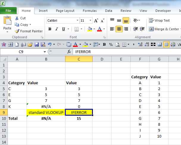
The second function is IFERROR and i more easy to use and overcomes all kinds of errors, not only #N/A.

The way to use it is like this: =IFERROR(VLOOKUP(item to be found,range,result column,0),0)

Keep on excelling!